Metis Data Science Bootcamp - Project 3
In the fifth week of the bootcamp, we were given the instructions for the third project. In this project, the students were asked to create a classification model that classifies labels based on certain features. For instance, if the data of different crimes is provided, one can train a model to classify the different types of crimes based on, for example, the neighborhood name, time and date. This post will illustrate my approach to tackle this particular problem.
Introduction
One of the most important pre-processing steps in some of image processing applications, like face detection and gesture recognition, is skin segmentation. Skin segmentation is challenging due to many areas of concern like the changing light intensity. My goal in this project is to take the different values of RGB colors of different pixels and classify them as skin pixels or non skin pixels.
Methodology
The approach that i have followed is summarized in the following figure:

These steps will be discussed in detail in the following subsections.
Step 1: Data Collecting
The dataset, skin segmentation dataset, was taken from UCI repository. This dataset includes the RGB values of pixels that were taken from face pictures of people of different ages, ethnic groups and genders. Each pixel is labeled as as either a skin pixel or non-skin pixel.
Step 2: Data Cleaning
In this step, null, Nan values and outliers were handled.
Step 3: Exploratory Data Analysis (EDA)
The pair plot for the different features is shown below.

Clearly, there is an overlap between the features but it is partial overlapping which means we can continue with the same features without worrying about removing any feature. Also, note that since we just have 3 features which are the values of the RGB colors, we can not remove any of them even if we have a complete overlapping between the features. Additionally, the scatter plots show that nonlinear model must be used.
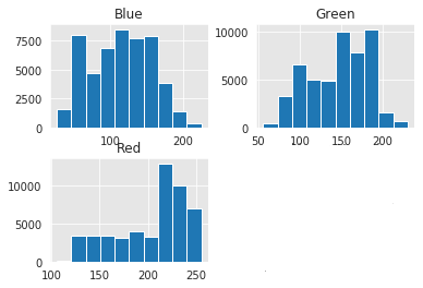
Now, let’s have a look at the histograms of the skin pixels and non-skin pixels.
Skin Pixels histograms:
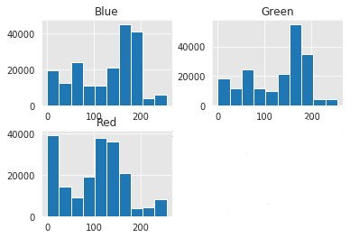
Non-Skin Pixels histograms:
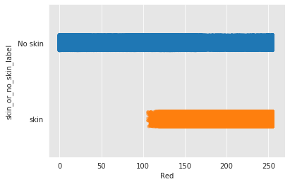
One interesting thing to notice in the histogram of the red color is that we can clearly say that any red value below 100 will be classified as a non-skin pixel. This tells us on initial thought that red color will be the most important feature in the classification model. The following figure illustrates the previously mentioned observation in a better way than the histogram.
Another interesting observation is that the number of skin pixels and non-skin pixels is different, so we have two options:
- Oversampling
- Undersampling
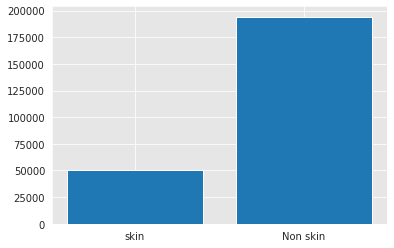
The dataset is not large, so oversampling is a better option. The oversampling is done using SMOTE.
Step 4: Modeling
Before creating any model, the data were split into training and test sets. Now, there are three things that must be noted before talking about the baseline model and the rest of the models. The first thing is that the train set is over-sampled, then the score of it is determined in all the models. The second thing is that when we do cross validation, we have to over-sample the 60 % train set and validate on the remaining 20% for each fold. The last thing is that the best possible hyper-parameters were chosen using cross validation that was applied using pipe-lining. The following figure illustrates how the typical cross validation is done.

- The Baseline Model: Logistic Regression Model
- solver= 'saga'
- penalty='elasticnet'
- l1_ratio=0.1
- C=100
- max_iter=1000
- The Second Model: Decision Trees Model
- criterion='entropy'
- max_depth=7
- Red (score = 0.65)
- Green (Score = 0.177)
- Blue (Score = 0.175)
- The Final Model: Random Forest
Logisitc regression model was chosen as the baseline model because it typically performs well in binary classification problems. The parameters for the model were as follows:
| Training F1-score | Cross-Validation F1-Score |
|---|---|
| 0.94 | 0.939 |
The last thing to note about this model is the coefficients. A simple of bar chart of the coefficients is shown below:
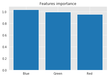
Well, this is strange. We expected red to have the highest impact on the model, but it did not.
The performance of the logistic regression was not bad, but we can always do better. Decision trees model was tuned by using the following parameters that were obtained by the pipeline:
| Training F1-score | Cross-Validation F1-Score | AUC |
|---|---|---|
| 1 | 0.9958 | 0.9972 |
The last thing to note about this model is the coefficients. The following list shows the features importance in descending order(Important first):
Now, these results confirms our initial assessment of the data since red is the most important feature.
Decision trees model provided excellent results, but can we do even better ? Yes ! random forest is the best performing model and its training and cross validation results are shown below:
| Training F1-score | Cross-Validation F1-Score | AUC |
|---|---|---|
| 1 | 0.9996 | 0.9999 |
The last thing to note about this model is the coefficients. A simple of bar chart of the coefficients is shown below:
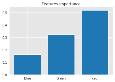
Now, these results confirms our initial assessment of the data as the previous model. However, it gives green higher score than the previous model. The testing results of this model will be illustrated in the following section